US baby names dataset¶

This notebook gives an example of Active Anomaly Detection with coniferest and US baby names dataset.

Developers of conferest:

Matwey Kornilov (MSU)
Vladimir Korolev
Konstantin Malanchev (LINCC Frameworks / CMU), notebook author

The tutorial is co-authored by Etienne Russeil (LPC)

Install and import modules¶

[1]:

%pip install 'coniferest[datasets]' pandas

Requirement already satisfied: pandas in /Users/hombit/.virtualenvs/coniferest/lib/python3.12/site-packages (2.3.0)
Requirement already satisfied: coniferest[datasets] in /Users/hombit/projects/supernovaAD/coniferest (0.0.11)
WARNING: coniferest 0.0.11 does not provide the extra 'datasets'
Requirement already satisfied: click in /Users/hombit/.virtualenvs/coniferest/lib/python3.12/site-packages (from coniferest[datasets]) (8.2.1)
Requirement already satisfied: joblib in /Users/hombit/.virtualenvs/coniferest/lib/python3.12/site-packages (from coniferest[datasets]) (1.5.1)
Requirement already satisfied: numpy in /Users/hombit/.virtualenvs/coniferest/lib/python3.12/site-packages (from coniferest[datasets]) (2.3.1)
Requirement already satisfied: scikit-learn<2,>=1 in /Users/hombit/.virtualenvs/coniferest/lib/python3.12/site-packages (from coniferest[datasets]) (1.7.0)
Requirement already satisfied: matplotlib in /Users/hombit/.virtualenvs/coniferest/lib/python3.12/site-packages (from coniferest[datasets]) (3.10.3)
Requirement already satisfied: onnxconverter-common in /Users/hombit/.virtualenvs/coniferest/lib/python3.12/site-packages (from coniferest[datasets]) (1.14.0)
Requirement already satisfied: scipy>=1.8.0 in /Users/hombit/.virtualenvs/coniferest/lib/python3.12/site-packages (from scikit-learn<2,>=1->coniferest[datasets]) (1.16.0)
Requirement already satisfied: threadpoolctl>=3.1.0 in /Users/hombit/.virtualenvs/coniferest/lib/python3.12/site-packages (from scikit-learn<2,>=1->coniferest[datasets]) (3.6.0)
Requirement already satisfied: python-dateutil>=2.8.2 in /Users/hombit/.virtualenvs/coniferest/lib/python3.12/site-packages (from pandas) (2.9.0.post0)
Requirement already satisfied: pytz>=2020.1 in /Users/hombit/.virtualenvs/coniferest/lib/python3.12/site-packages (from pandas) (2025.2)
Requirement already satisfied: tzdata>=2022.7 in /Users/hombit/.virtualenvs/coniferest/lib/python3.12/site-packages (from pandas) (2025.2)
Requirement already satisfied: six>=1.5 in /Users/hombit/.virtualenvs/coniferest/lib/python3.12/site-packages (from python-dateutil>=2.8.2->pandas) (1.17.0)
Requirement already satisfied: contourpy>=1.0.1 in /Users/hombit/.virtualenvs/coniferest/lib/python3.12/site-packages (from matplotlib->coniferest[datasets]) (1.3.2)
Requirement already satisfied: cycler>=0.10 in /Users/hombit/.virtualenvs/coniferest/lib/python3.12/site-packages (from matplotlib->coniferest[datasets]) (0.12.1)
Requirement already satisfied: fonttools>=4.22.0 in /Users/hombit/.virtualenvs/coniferest/lib/python3.12/site-packages (from matplotlib->coniferest[datasets]) (4.58.4)
Requirement already satisfied: kiwisolver>=1.3.1 in /Users/hombit/.virtualenvs/coniferest/lib/python3.12/site-packages (from matplotlib->coniferest[datasets]) (1.4.8)
Requirement already satisfied: packaging>=20.0 in /Users/hombit/.virtualenvs/coniferest/lib/python3.12/site-packages (from matplotlib->coniferest[datasets]) (25.0)
Requirement already satisfied: pillow>=8 in /Users/hombit/.virtualenvs/coniferest/lib/python3.12/site-packages (from matplotlib->coniferest[datasets]) (11.2.1)
Requirement already satisfied: pyparsing>=2.3.1 in /Users/hombit/.virtualenvs/coniferest/lib/python3.12/site-packages (from matplotlib->coniferest[datasets]) (3.2.3)
Requirement already satisfied: onnx in /Users/hombit/.virtualenvs/coniferest/lib/python3.12/site-packages (from onnxconverter-common->coniferest[datasets]) (1.17.0)
Requirement already satisfied: protobuf==3.20.2 in /Users/hombit/.virtualenvs/coniferest/lib/python3.12/site-packages (from onnxconverter-common->coniferest[datasets]) (3.20.2)
Note: you may need to restart the kernel to use updated packages.

[2]:

import datasets
import matplotlib.pyplot as plt
import numpy as np
import pandas as pd
import requests
from coniferest.pineforest import PineForest
from coniferest.isoforest import IsolationForest
from coniferest.pineforest import PineForest
from coniferest.session import Session
from coniferest.session.callback import TerminateAfter, prompt_decision_callback, Label

/Users/hombit/.virtualenvs/coniferest/lib/python3.12/site-packages/tqdm/auto.py:21: TqdmWarning: IProgress not found. Please update jupyter and ipywidgets. See https://ipywidgets.readthedocs.io/en/stable/user_install.html
  from .autonotebook import tqdm as notebook_tqdm

Data preparation¶

Download data and put into a single data frame

[3]:

%%time

# Hugging Face dataset constructed from
# https://www.ssa.gov/OACT/babynames/state/namesbystate.zip
dataset = datasets.load_dataset("snad-space/us-names-by-state")
raw = dataset['train'].to_pandas()

raw

Downloading data: 100%|██████████| 51/51 [00:01<00:00, 41.41files/s]
Generating train split: 100%|██████████| 6600640/6600640 [00:02<00:00, 2268886.44 examples/s]

CPU times: user 3.14 s, sys: 970 ms, total: 4.1 s
Wall time: 5.64 s

[3]:

	State	Gender	Year	Name	Count
0	AK	F	1910	Mary	14
1	AK	F	1910	Annie	12
2	AK	F	1910	Anna	10
3	AK	F	1910	Margaret	8
4	AK	F	1910	Helen	7
...	...	...	...	...	...
6600635	WY	M	2024	Royce	5
6600636	WY	M	2024	Spencer	5
6600637	WY	M	2024	Truett	5
6600638	WY	M	2024	Wylder	5
6600639	WY	M	2024	Xander	5

6600640 rows × 5 columns

Let’s load the data and transform it into a feature matrix where each column is the number (normalized by peak value) of US citizens that got this name in a given year. We apply few quality filter. We require the name to appear at least 10000 times over the full time range, this will prevent noisy data from names that are barely used.

Optionally, we use first few Fourier terms to better detect “bumps” and “waves” in the time-series.

[4]:

%%time

WITH_FFT = True

all_years = np.unique(raw['Year'])
all_names = np.unique(raw['Name'])

# Accumulate names over states and genders
counts = raw.groupby(
    ['Name', 'Year'],
).apply(
    lambda df: df['Count'].sum(),
    include_groups=False,
)

# Transform to a data frame where names are labels, years are columns and counts are values (features)
years = [f'year_{i}' for i in all_years]
year_columns = pd.DataFrame(data=0.0, index=all_names, columns=years)
for name, year in counts.index:
    year_columns.loc[name, f'year_{year}'] = counts.loc[name, year]

# Account for total population changes
trend = year_columns.sum(axis=0)
detrended = year_columns / trend

# Normalise and filter
norm = detrended.apply(lambda column: column / detrended.max(axis=1))
filtered = norm[year_columns.sum(axis=1) >= 10_000]

if WITH_FFT:
    # Fourier-transform, normalize by zero frequency and get power-spectrum for few lowest frequencies
    power_spectrum = np.square(np.abs(np.fft.fft(filtered)))
    power_spectrum_norm = power_spectrum / power_spectrum[:, 0, None]
    power_spectrum_low_freq = power_spectrum_norm[:, 1:21]
    frequencies = [f'freq_{i}' for i in range(power_spectrum_low_freq.shape[1])]
    power = pd.DataFrame(data=power_spectrum_low_freq, index=filtered.index, columns=frequencies)

    # Concatenate time-series data and power spectrum
    final = pd.merge(filtered, power, left_index=True, right_index=True)
else:
    # Use time-series data
    final = filtered

final

CPU times: user 32 s, sys: 492 ms, total: 32.5 s
Wall time: 32.9 s

[4]:

	year_1910	year_1911	year_1912	year_1913	year_1914	year_1915	year_1916	year_1917	year_1918	year_1919	...	freq_10	freq_11	freq_12	freq_13	freq_14	freq_15	freq_16	freq_17	freq_18	freq_19
Aaliyah	0.000000	0.000000	0.000000	0.000000	0.000000	0.000000	0.000000	0.000000	0.000000	0.000000	...	0.007815	0.011471	0.009205	0.002661	0.000384	0.003367	0.004686	0.002152	0.000062	0.000980
Aaron	0.045721	0.053748	0.062029	0.077329	0.074982	0.065564	0.066903	0.066013	0.065492	0.066256	...	0.000203	0.000332	0.000003	0.000209	0.000003	0.000213	0.000325	0.000083	0.000084	0.000259
Abbey	0.000000	0.000000	0.000000	0.000000	0.000000	0.000000	0.000000	0.000000	0.000000	0.000000	...	0.003283	0.002742	0.000650	0.000279	0.000762	0.000680	0.000231	0.000050	0.000016	0.000096
Abbie	0.359963	0.269810	0.306465	0.464630	0.215549	0.302426	0.349251	0.307615	0.197811	0.346344	...	0.000792	0.000478	0.000180	0.000260	0.001956	0.000199	0.000055	0.000111	0.000089	0.000495
Abbigail	0.000000	0.000000	0.000000	0.000000	0.000000	0.000000	0.000000	0.000000	0.000000	0.000000	...	0.002717	0.001827	0.001172	0.001199	0.001423	0.001123	0.000468	0.000081	0.000061	0.000128
...	...	...	...	...	...	...	...	...	...	...	...	...	...	...	...	...	...	...	...	...	...
Zelma	0.932474	1.000000	0.729411	0.723821	0.652394	0.669621	0.600106	0.576397	0.536196	0.576366	...	0.012596	0.010955	0.009435	0.007556	0.005983	0.005520	0.005827	0.005979	0.005959	0.006366
Zion	0.000000	0.000000	0.000000	0.000000	0.000000	0.000000	0.000000	0.000000	0.000000	0.000000	...	0.022560	0.009141	0.002182	0.006346	0.010988	0.008036	0.002212	0.001621	0.005530	0.006818
Zoe	0.009245	0.000000	0.003225	0.000000	0.001845	0.002542	0.004275	0.004373	0.002134	0.001221	...	0.010147	0.009064	0.004659	0.001311	0.001038	0.002035	0.002939	0.003169	0.002656	0.002130
Zoey	0.000000	0.000000	0.000000	0.000000	0.000000	0.000000	0.000000	0.000000	0.000000	0.000000	...	0.010202	0.010542	0.008716	0.005578	0.002431	0.000437	0.000107	0.000786	0.001459	0.001728
Zuri	0.000000	0.000000	0.000000	0.000000	0.000000	0.000000	0.000000	0.000000	0.000000	0.000000	...	0.041216	0.032491	0.029391	0.026944	0.022914	0.018828	0.013810	0.008968	0.007011	0.007291

2337 rows × 135 columns

Plotting function

[5]:

def basic_plot(idx):
    cols = [col.startswith('year') for col in final.columns]
    all_years = [int(col.removeprefix('year_')) for col in final.columns[cols]]

    if isinstance(idx, str):
        counts = final.loc[idx][cols]
        title = idx
    else:
        counts = final.iloc[idx][cols]
        title = final.iloc[idx].name

    plt.plot(all_years, counts.values)
    # plt.ylim(-0.1, 1.1)
    plt.title(title)
    plt.xlabel('Year')
    plt.ylabel('Count')
    plt.show()
    return

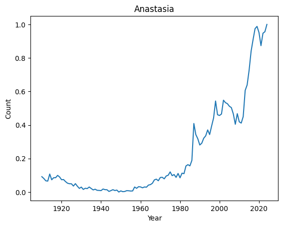
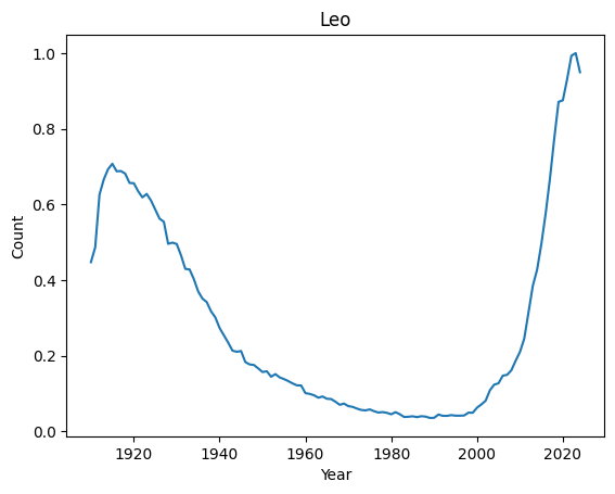
We can now easily look at the evolution of a given name over the years

[6]:

print(len(final))
basic_plot('Anastasia')
basic_plot('Leo')

Classical anomaly detection¶

[7]:

model = IsolationForest(random_seed=1, n_trees=1000)
model.fit(np.array(final))
scores = model.score_samples(np.array(final))
ordered_scores, ordered_index = zip(*sorted(zip(scores, final.index)))

print(f"Top 10 weirdest names : {ordered_index[:10]}")
print(f"Top 10 most regular names : {ordered_index[-10:]}")

Top 10 weirdest names : ('Manuel', 'Marshall', 'Alfonso', 'Vincent', 'Margarita', 'Byron', 'Rudy', 'Benito', 'Peter', 'Ruben')
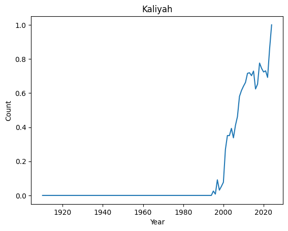
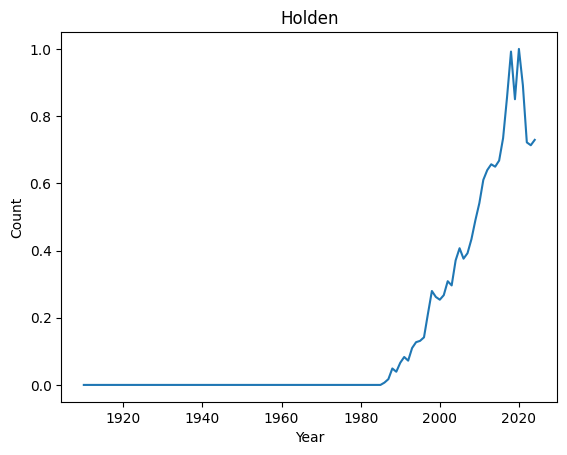
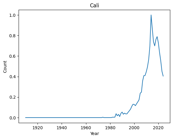
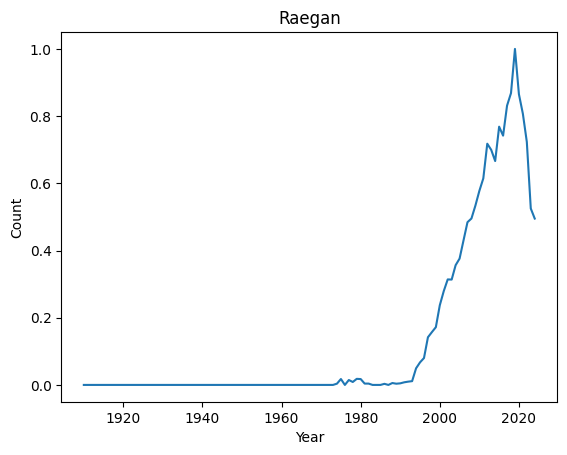
Top 10 most regular names : ('Kian', 'Jayla', 'Kenzie', 'Ibrahim', 'Teagan', 'Phoenix', 'Kaliyah', 'Holden', 'Cali', 'Raegan')

Let’s have a look at their distributions

[8]:

for normal in ordered_index[-4:]:
    basic_plot(normal)

[9]:

for weird in ordered_index[:4]:
    basic_plot(weird)

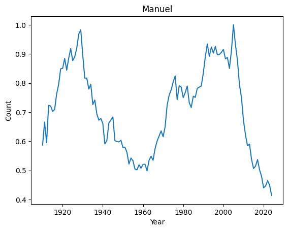
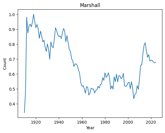
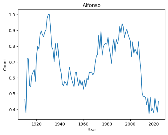
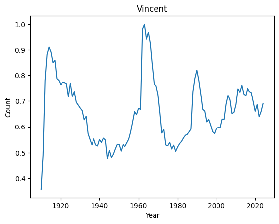
It seems that anomalies are either very localised peak or very recent trending names.

Active Anomaly Detection¶

First, we need a function helping us to make a decision.

Comment dummy decision function and uncomment interactive one¶

[10]:

# Comment
def help_decision(metadata, data, session):
    """Dummy, says YES to everything"""
    return Label.ANOMALY

### UNCOMMENT
# def help_decision(metadata, data, session):
#     """Plots data and asks expert interactively"""
#     basic_plot(metadata)
#     return prompt_decision_callback(metadata, data, session)

Let’s create a model and run a session

Let’s run PineForest and say YES every time we see a recent growth

[11]:

model = PineForest(
    # Number of trees to use for predictions
    n_trees=256,
    # Number of new trees to grow for each decision
    n_spare_trees=768,
    # Fix random seed for reproducibility
    random_seed=0,
)
session = Session(
    data=final,
    metadata=final.index,
    model=model,
    decision_callback=help_decision,
    on_decision_callbacks=[
        TerminateAfter(10),
    ],
)
session.run()

[11]:

<coniferest.session.Session at 0x12f081b20>

Wow! Good almost 100% of the behavior we were looking for

Now we can run it again and say YES every time we see a sharp peak

[12]:

model = PineForest(
    # Number of trees to use for predictions
    n_trees=256,
    # Number of new trees to grow for each decision
    n_spare_trees=768,
    # Fix random seed for reproducibility
    random_seed=0,
)
session = Session(
    data=final,
    metadata=final.index,
    model=model,
    decision_callback=help_decision,
    on_decision_callbacks=[
        TerminateAfter(20),
    ],
)
session.run()

[12]:

<coniferest.session.Session at 0x12f1930b0>

PineForest learns the profile interesting for the user and outputs it.

Try to change Pineforest hyperparameters and see how results change. Try different random seeds and number of trees.

[ ]:

US baby names dataset¶

Install and import modules¶

Data preparation¶

Classical anomaly detection¶

Active Anomaly Detection¶

Comment dummy decision function and uncomment interactive one¶

coniferest

Navigation

Related Topics